Classification with imbalanced data

Mohsen is a seasoned optimization expert who takes a principal role in implementing and validating data science and artificial intelligence models.
PhD in AI • Senior Consultant #MachineLearning #DataScience @BasicFitNL Previous: @Shell @LINKITGroup @FU_Mashhad @TUDelft @ErasmusMC @DanielDenHoed @CapgeminiNL @KLM
Consider the problem of predicting late passengers at the airport. Based on some statistics, only around 8% of passengers are considered late. Assuming the availability of good features like Age, Gender, Nationality, Country of residence, Walking distance from the baggage drop-off point to the gate, etc., the easy solution would be to build a random forest and train it using let’s say 80% of the available data set. The other 20% of data is reserved for testing. What does it mean If the classifier gets an accuracy of 92%? Bad.
So the question that comes to mind is why does it happen, and how to handle imbalanced classification problems?
The answer to the first question, why does it happen, is a simple one. When the problem at hand is imbalanced, the ML algorithm has little information about the minority class. So it’s not a simple task to come up with a list of features that are informative to discriminate the classes.
For the second question, how to handle the problem, one may provide several answers, mainly supported by conceptual reasoning and simulated results. We shall review a number of them in this article. Without loss of generality, binary classification is considered here.
Approaches to deal with imbalanced data sets
The skewed class distribution is quantized by the imbalance ratio (IR) and is defined as the ratio of the number of instances in the majority class to the number of examples in the minority class.
The approaches are categorized into two groups: the internal approaches and external approaches. While the former group aims at creating new algorithms or modifying the existing ones, the latter acts on the data by resampling to diminish the effect caused by class imbalance.
Internal approaches
Internal approaches modify the existing algorithms or create new ones equipped with approaches to handle imbalanced classification problems. They may adapt the decision threshold to create a bias toward the minority class. Or may modify the cost function to compensate the minority class.
External approaches
This group acts on the data rather than the learning method. Their advantage over internal approaches is their independence from the classifier used. One of the methods to deal with imbalance classification problems is the Data Sampling Method, each with its characteristics, strengths, and weaknesses. These techniques assume that a fully balanced dataset can be attained. Data Sampling methods transform the imbalanced data set into balanced data by under-sampling the majority class, over-sampling the minority class, and/or generating synthesized data to bring the class ratio to 50:50. A very well-known representative of the latter method is known as Synthetic Minority Oversampling Technique or SMOTE. Although several studies have shown little to no difference between these data sampling techniques, we shall review all three of them.
Random Undersampling (RUS)
Random Undersampling (RUS) tries to balance the two classes by reducing the size of the majority class accomplished by removing instances of the majority instance. Observations from the majority class are selected and removed from the database at random, and the process continues until the desired class ratio is reached.
Random Oversampling (ROS)
As you might have already guessed, Random Oversampling balances the dataset by increasing the size of the minority class. The desired class ratio is achieved by duplicating samples from the minority class. The items to be duplicated are selected at random.
ROS, when compared to RUS, ensures efficient use of information and prevents information loss. On the other hand, the chance of overfitting is high when using random oversampling, meaning that the training accuracy may be improved at the cost of lower performance on the test set.
Synthetic Data Generation
This group of techniques is a type of oversampling with the aim of balancing the classes by generating synthetic data. The most widely used and well-known member of this group is the synthetic minority oversampling technique (SMOTE). This set of algorithms oversamples the minority class by the use of k-nearest neighbors.
Cost-sensitive Learning (CSL)
Cost-sensitive learning framework takes advantage of both External approaches (by adding costs to instances) and Internal approaches (by modifying the internal learning process to accept costs). In this framework, the cost of misclassification of the minority class is higher in comparison to the cost of misclassification of the majority class. The cost matrix is composed of four quadrants, that resemble the confusion matrix. The penalty for True Positive and True Negatives is zero, thus the total cost is the weights sum of \(C_{FN}\) and \(C_{FP}\) and may be computed using the following equation:
$$C_T=C_{FN}∗||FN||+C_{FP}∗||FP||$$
where \(||FN||\) is the number of false negatives (positive examples wrongly predicted) and \(||FP||\) is the number of False negatives (negative observations wrongly predicted). Depending on the application, \(C_{FN} > C_{FP} \) or \(C_{FP} > C_{FN}\).
Selection of performance metrics
ROC curve and how to plot it?
In most cases, the output of the classifier is a score (and not the probability) bounded in the range of 0 and 1. If the output is less than a threshold \(\theta\) then we would say the instance belongs to class \(-1\), otherwise, it belongs to class $1$. Note that \(\theta\) is bounded between the max and min value of the output of the model, which might be 0 and 1.
For every \(\theta\), the true positive ratio (TPR) and false positive ratio (FPR) can be computed. TPR is the ratio of correct positive results to all positive samples available during the test. FPR is a number of incorrect positive results to all negative samples available during the test.
Now every choice for \(\theta\) corresponds to a point in the ROC Space. In ROC Space the X-axis specifies the False Positive Rate (also known as Specificity) and the Y-axis represents the True Positive Rate (also known as Sensitivity). So the y-axis reflects the proportion of actual positives that are correctly classified as positives.
The area under the ROC curve is known as the AUC (area under curve) or c-statistic. In the ML community AUC statistic is the most often used metric for model comparison.
Note that the area between the ROC curve and the no-discrimination line (the diagonal line) is known as the Gini Coefficient.
ROC curves are known to be insensitive to class balance, hence a good choice for imbalanced datasets.
Further Reading
There is a wealth of literature on classifiers in imbalanced domains, along with a comprehensive exploration of the challenges they pose. For readers interested in delving deeper into the topic, below is a list of challenges and references that address them.
Noisy data and imbalanced domains [Knowledge discovery from imbalanced and noisy data, 2009].
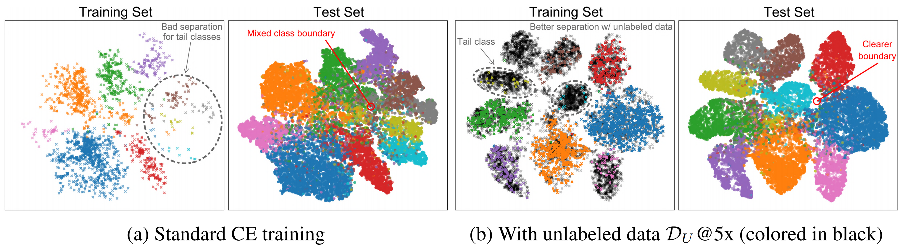
Dataset shift: A very well-known concept in ML space that refers to variations in the distribution of data between the training and test datasets [The balancing trick: Optimized sampling of imbalanced datasets—A brief survey of the recent State of the Art, 2020] and [Rethinking the Value of Labels for Improving Class-Imbalanced Learning, 2020]
Summary
While Imbalanced classification is a common issue in many ML and data science, there is no single-bullet solution to address the challenge. Strategies such as resampling and the use of various evaluation metrics have the potential to address the challenges. What remains important is continuously monitoring the models we have in production and being cautious of potential data drifts.
Behind every great product there is a great product manager. That is why there are so few great products out there.
A cool data scientist, Delft
Cover Image Credit: Chris Wren and Kenn Brown/mondoworks.